The simulations discussed above seem to indicate that there is a
solid-solid transition even in the limit where  .
At first sight this seems surprising, because one would not expect an
infinitely narrow potential well to affect the phase behavior at
finite temperature. However, at close packing, even an infinitely
narrow potential will give a finite contribution to the potential
energy. Surprisingly, it turns out that it is possible to perform
simulations of the phase behavior in the limit
.
At first sight this seems surprising, because one would not expect an
infinitely narrow potential well to affect the phase behavior at
finite temperature. However, at close packing, even an infinitely
narrow potential will give a finite contribution to the potential
energy. Surprisingly, it turns out that it is possible to perform
simulations of the phase behavior in the limit  .
To see how this can be achieved, it is convenient to consider first
the more general case that
.
To see how this can be achieved, it is convenient to consider first
the more general case that  is finite. In the dense
crystalline solid, any given particle i is constrained to move in
the vicinity of its lattice site - i.e. its average position -
is finite. In the dense
crystalline solid, any given particle i is constrained to move in
the vicinity of its lattice site - i.e. its average position -
 . In that case, we can re-express the potential energy as a
function of the displacement
. In that case, we can re-express the potential energy as a
function of the displacement  of the particles, from their
respective lattice sites:
of the particles, from their
respective lattice sites:  .
The potential energy of a pair of particles can then be written as
.
The potential energy of a pair of particles can then be written as
where we have used the obvious notation  .
For nearest neighbors,
.
For nearest neighbors,  at
close packing. At lower densities,
at
close packing. At lower densities,  where a has been defined in eqn.
3.6. The
potential energy of a pair of square-well particles is a function of
where a has been defined in eqn.
3.6. The
potential energy of a pair of square-well particles is a function of
 ,
We can now express
,
We can now express  in terms of
  and
and
 . This yields the following result for
where  is a unit vector in the direction of
  and
and  .
In the limit
.
In the limit  takes on a very
simple form
takes on a very
simple form
In this limit, the square-well model is equivalent to a lattice model,
with a fixed, but arbitrary lattice spacing as shown in figure 3.4.
The state at every lattice point i is characterized by a
scaled displacement vector  .
Note that a finite
.
Note that a finite  corresponds to an infinitesimal real
displacement
corresponds to an infinitesimal real
displacement  . The nearest-neighbor
interaction is a function of
. The nearest-neighbor
interaction is a function of  . Clearly, the density in the original square-well model
now only enters in the problem through the parameter
. Clearly, the density in the original square-well model
now only enters in the problem through the parameter  . We
can now perform Monte Carlo simulations on this lattice model
by moving a randomly selected atom i from its initial scaled
displacement
. We
can now perform Monte Carlo simulations on this lattice model
by moving a randomly selected atom i from its initial scaled
displacement  to the trial displacement
  in
such a way that
microscopic reversibility is satisfied.
in
such a way that
microscopic reversibility is satisfied.
Knowledge of the new scaled displacement of atom i is sufficient to compute the change in potential energy associated with the trial move, using eqns
3.7 - 3.9 above.
We now use the conventional Metropolis rule to accept or reject the trial
move.
By combining the results of a series of simulations for a range
of values of  and a range of temperatures (twenty
temperatures and thirty
and a range of temperatures (twenty
temperatures and thirty  values for every temperature) with the
hard-sphere equation of state near close packing [57], we can
compute the free energy of this model system as a function of temperature
and volume by thermodynamic integration and construct the solid-solid
phase diagram in the limit
values for every temperature) with the
hard-sphere equation of state near close packing [57], we can
compute the free energy of this model system as a function of temperature
and volume by thermodynamic integration and construct the solid-solid
phase diagram in the limit  =0.
In the
=0.
In the  plane, the binodal would simply be a vertical line
segment at close packing ending in a critical point.
It is more convenient to plot the binodal as a function of
plane, the binodal would simply be a vertical line
segment at close packing ending in a critical point.
It is more convenient to plot the binodal as a function of  .
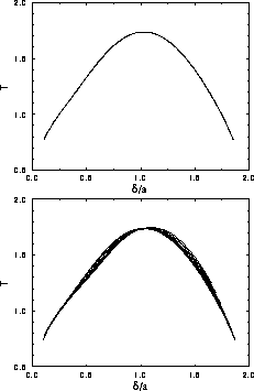
In figure 3.5, the solid-solid binodal is plotted in the
.
In figure 3.5, the solid-solid binodal is plotted in the
 plane. As can be seen from the figure the critical
temperature is indeed finite. Moreover, the binodal becomes quite
symmetric in this representation compared to figure 3.2.
plane. As can be seen from the figure the critical
temperature is indeed finite. Moreover, the binodal becomes quite
symmetric in this representation compared to figure 3.2.
It is interesting to consider the square-well solid at finite
 in terms of the lattice model described above. As
can be seen from eqn.
3.7 and eqn.
3.8, the
potential energy now is a function not only of
in terms of the lattice model described above. As
can be seen from eqn.
3.7 and eqn.
3.8, the
potential energy now is a function not only of  and
and  but also of
  . If the free energy of
the system is an analytic function of
. If the free energy of
the system is an analytic function of  , we could
expand in powers of it around the limit
, we could
expand in powers of it around the limit  =0. However,
the solid-solid transition only occurs for
=0. However,
the solid-solid transition only occurs for  0.06.
Hence,
0.06.
Hence,  is always a small parameter. It is therefore
likely that the phase diagram of the square-well model, when plotted
as a function of
is always a small parameter. It is therefore
likely that the phase diagram of the square-well model, when plotted
as a function of  differs only little from the behavior
in the limit
differs only little from the behavior
in the limit  . As can be seen from
figure 3.5 this is indeed the case.
. As can be seen from
figure 3.5 this is indeed the case.
It is interesting to point out the relation between the square-well
model in the limit  =0 and the adhesive hard-sphere
model proposed by Baxter [51].
The adhesive hard-sphere model is obtained from the square-well model
by considering the limit
=0 and the adhesive hard-sphere
model proposed by Baxter [51].
The adhesive hard-sphere model is obtained from the square-well model
by considering the limit 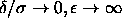 such that
  . This limiting procedure results in a model that has
a finite second virial coefficient at finite temperature. Usually,
the ratio of the second virial coefficient of the adhesive
hard-sphere to that of ``non-sticky'' hard spheres is used to relate
the parameter
. This limiting procedure results in a model that has
a finite second virial coefficient at finite temperature. Usually,
the ratio of the second virial coefficient of the adhesive
hard-sphere to that of ``non-sticky'' hard spheres is used to relate
the parameter  to observable quantities:

The adhesive hard sphere system has been studied extensively, both
theoretically [58,59,60] and
numerically [61,62].
In particular, the liquid-vapor critical point of this model has been
predicted to occur at  0.097 [58].
However, if we identify the adhesive hard-sphere model with the
square-well model in the limit
0.097 [58].
However, if we identify the adhesive hard-sphere model with the
square-well model in the limit  , then
the present simulations show that this model already has a
solid-solid transition for
, then
the present simulations show that this model already has a
solid-solid transition for 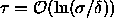 ,
i.e. for
,
i.e. for  .
At all finite temperatures (finite
.
At all finite temperatures (finite  ) the only stable phases are
the close-packed solid and the infinitely dilute gas. Hence, all
other phases of the adhesive hard-sphere model are, at best, metastable.
In fact, Stell [63] has already indicated that the
monodisperse adhesive hard-sphere model is pathological because the
) the only stable phases are
the close-packed solid and the infinitely dilute gas. Hence, all
other phases of the adhesive hard-sphere model are, at best, metastable.
In fact, Stell [63] has already indicated that the
monodisperse adhesive hard-sphere model is pathological because the
 virial coefficient diverges. This divergence could be removed by
introducing a slight size polydispersity into the model. Such
polydispersity would also affect the solid-solid transition. In fact,
a rough estimate of the phase-diagram suggest that in that case, the
solid-fluid transition occurs at finite
virial coefficient diverges. This divergence could be removed by
introducing a slight size polydispersity into the model. Such
polydispersity would also affect the solid-solid transition. In fact,
a rough estimate of the phase-diagram suggest that in that case, the
solid-fluid transition occurs at finite  , and hence the phase
diagram of the slightly polydisperse adhesive hard sphere model is
non-trivial.
, and hence the phase
diagram of the slightly polydisperse adhesive hard sphere model is
non-trivial.
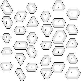
 .
The lines of the hexagons give the momentary boundary of the cell to
which a particle is confined.
All the cells are scaled up to finite size, as the cells are infinitely
small in the limit
.
The lines of the hexagons give the momentary boundary of the cell to
which a particle is confined.
All the cells are scaled up to finite size, as the cells are infinitely
small in the limit  .
The cell boundaries will change position if the nearest neighbors move.
The arrows give the particle displacement from their original lattice
positions.
In the shaded area the particles are within the interaction range of
their neighbors.
.
The cell boundaries will change position if the nearest neighbors move.
The arrows give the particle displacement from their original lattice
positions.
In the shaded area the particles are within the interaction range of
their neighbors.


 plane (see text). The upper figure shows the binodal in
the limit
plane (see text). The upper figure shows the binodal in
the limit  =0, while the bottom figure shows that all
the scaled binodals for finite
=0, while the bottom figure shows that all
the scaled binodals for finite  0.07 very nearly
coincide with the binodal for
0.07 very nearly
coincide with the binodal for  =0.
=0.