and has an
attractive interaction with a characteristic range
and has an
attractive interaction with a characteristic range  , outside
the repulsive core. The functional form of the square-well potential is:
, outside
the repulsive core. The functional form of the square-well potential is:
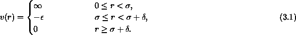
The square-well model provides a very simple description of particles
interacting through a pair potential that is harshly repulsive at
distances less than a characteristic diameter and has an
attractive interaction with a characteristic range , outside
the repulsive core. The functional form of the square-well potential is:
where  is the depth of the attractive well.
In order to compute the phase diagram of the square-well system, we first
must determine the dependence of the Helmholtz free energy of the solid on
density and temperature. As the free energy of the solid cannot be measured
directly in a Monte Carlo simulation, we use thermodynamic integration to
relate the free energy of the square-well solid to that of a reference
hard-sphere solid
at the same density [53].
is the depth of the attractive well.
In order to compute the phase diagram of the square-well system, we first
must determine the dependence of the Helmholtz free energy of the solid on
density and temperature. As the free energy of the solid cannot be measured
directly in a Monte Carlo simulation, we use thermodynamic integration to
relate the free energy of the square-well solid to that of a reference
hard-sphere solid
at the same density [53].
where  is the reduced well-depth
  and
<E>, the average internal energy of the system, a quantity that
can be measured in a Monte Carlo NVT simulation.
The instantaneous energy is equal to the number of pairs of atoms
and
<E>, the average internal energy of the system, a quantity that
can be measured in a Monte Carlo NVT simulation.
The instantaneous energy is equal to the number of pairs of atoms
 that are within the range of the potential times the depth of
potential well
that are within the range of the potential times the depth of
potential well  . The dimensionless free energy per particle
now is simply
. The dimensionless free energy per particle
now is simply
The free energy of the three dimensional hard-sphere solid  is
well known and can be accurately represented using the analytical
form for the equation of state
proposed by Hall [54]. In two dimensions the free energy of the
hard-disk
``solid'' can be obtained from simulations done by Alder et al. [55].
is
well known and can be accurately represented using the analytical
form for the equation of state
proposed by Hall [54]. In two dimensions the free energy of the
hard-disk
``solid'' can be obtained from simulations done by Alder et al. [55].
The presence of a first-order phase transition in the square-well
solid is signaled by the fact that
the Helmholtz free energy becomes a non-convex function of the volume. The
densities of the coexisting phases can then be determined by a standard
double-tangent construction.
In order to map out the phase diagram of the square-well solid over a
wide range of densities and temperatures as a function of the width
of the attractive well, several thousand independent simulations were
required. To keep the computational costs within bounds, we
chose to simulate a relatively small system.
With a small system size, finite-size effects are expected, in
particular in the vicinity of a critical point. However, away from critical
points finite-size effects should be so small that they will not affect
the conclusions that we draw below.
In what follows, we use reduced units, such that
 is the unit of temperature,
and
is the unit of temperature,
and  , the hard-core diameter of the particles, is the unit of length.
For the two dimensional case, the simulation parameters were as follows:
All simulated systems consisted of a periodic triangular lattice of
200 disks, placed in a rectangular simulation box with side ratio  .
The densities ranged from
.
The densities ranged from  =0.8 which is below the hard-disk
``melting point'' to
=0.8 which is below the hard-disk
``melting point'' to  =1.154 which is almost at close packing
(
=1.154 which is almost at close packing
( ). The temperature of the system was varied in the range
0
). The temperature of the system was varied in the range
0 2, in steps of 0.1.
Simulations were performed for
2, in steps of 0.1.
Simulations were performed for
 =0.01, 0.02, 0.03, 0.04, 0.05, 006 and 0.07.
All simulations on the three-dimensional system were performed on a
face-centered cubic ( fcc)
solid consisting of 108 particles. This is presumably the stable
solid structure for hard-spheres  and for the square-well
model with short-ranged attraction ( i.e. only nearest neighbor interaction).
The simulation box was chosen to be cubic and periodic boundaries were
applied. The densities ranged from
and for the square-well
model with short-ranged attraction ( i.e. only nearest neighbor interaction).
The simulation box was chosen to be cubic and periodic boundaries were
applied. The densities ranged from  =0.9 which is below the hard-sphere
melting point to
=0.9 which is below the hard-sphere
melting point to  =1.414 which is almost at close packing
(
=1.414 which is almost at close packing
( ). The temperature of the system was varied over
the same range as in the two dimensional case.
Simulations were performed for
). The temperature of the system was varied over
the same range as in the two dimensional case.
Simulations were performed for  =0.001, 0.002,
0.003, 0.004, 0.005, 0.01, 0.02, 0.03, 0.04, 0.05 and 0.06.
For every value of the well-width
=0.001, 0.002,
0.003, 0.004, 0.005, 0.01, 0.02, 0.03, 0.04, 0.05 and 0.06.
For every value of the well-width  in both the two and three
dimensional case,
we performed some 1000 MC simulations of 20000 cycles each.
in both the two and three
dimensional case,
we performed some 1000 MC simulations of 20000 cycles each.
In order to perform the double-tangent construction on the Helmholtz
free energy, all simulation data
were fitted to an analytical function of  ,
,  and T.
We chose to use a fit function that reproduced the correct limiting
behavior at close packing. In particular, for the 2D case, we used
the following functional form
and T.
We chose to use a fit function that reproduced the correct limiting
behavior at close packing. In particular, for the 2D case, we used
the following functional form
and in the three dimensional case we chose the following form
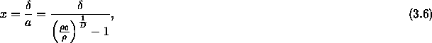
The parameter x in eqn.
3.4 and eqn.
3.5
is defined as the ratio of well width d to the distance a, that
characterizes the expansion of the solid from close packing:
 , where
  is the average nearest
neighbor distance and
is the average nearest
neighbor distance and  is the hard sphere diameter. x is
simply related to the density, through:
is the hard sphere diameter. x is
simply related to the density, through:
where D is the dimensionality of the system. For large x - i.e. near close packing - the functions given in eqn. 3.4 and eqn. 3.5 go to the value of half the number of nearest neighbors per particle.
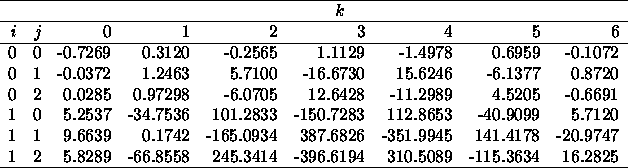
| Table: | Best fit coefficients  for eqn.
3.4 for eqn.
3.4 |
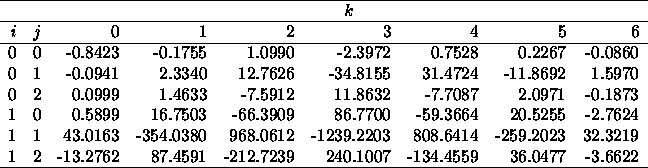
| Table: | Best fit coefficients  for eqn.
3.5 for eqn.
3.5 |
The coefficients of the best fits to the numerical data are given in tables 3.2.1 and 3.2.1. These fits reproduce the numerical data to within the statistical error. Using the functional forms given by eqn. 3.4 and eqn. 3.5 to represent the numerical data, we computed the free energy of the solid as a function of temperature and volume, using eqn. 3.3. The resulting free energy functions were checked for possible non-convex dependence on the volume V. Whenever such an indication of a first-order phase transition was found, the densities of the coexisting phases were determined by equating the pressures and chemical potentials in both phases using the standard double tangent construction. The critical temperature of the solid-solid coexistence curve was estimated to be the point where the free energy curve first developed an inflection point. Of course, this estimate is likely to depend somewhat on the system size. Moreover, the analytical form of eqn. 3.4 and eqn. 3.5 forces the classical (mean-field) critical behavior on the solid-solid binodal. We have not attempted to study the true critical behavior of the solid-solid transition.