Next: Conclusion Up: Binary mixtures ofhard Previous: Introduction
Next: Conclusion
Up: Binary mixtures ofhard
Previous: Introduction
To study the possibility of
phase separation in a
rod-plate mixture we performed Gibbs-ensemble Monte Carlo simulations
[31,32,33] of a binary mixture of ellipsoids of revolution. We chose
an aspect ratio of  =15, high enough to ensure biaxiality at
relative low density and yet small enough to obviate the need for
large system sizes. In the Monte Carlo simulations, we used the
Vieillard-Barron overlap criterion in combination with the
Perram-Wertheim test for non-overlap[77]. The Gibbs-ensemble
MC simulations were performed for a system of 1200 prolate and 800
oblate ellipsoids. This slightly asymmetric overall
composition was chosen to ensure that the sizes of the two simulation boxes
in the GEMC simulations do not become too different.
As is usual
in the study of mixtures, the total pressure of the system was kept constant.
=15, high enough to ensure biaxiality at
relative low density and yet small enough to obviate the need for
large system sizes. In the Monte Carlo simulations, we used the
Vieillard-Barron overlap criterion in combination with the
Perram-Wertheim test for non-overlap[77]. The Gibbs-ensemble
MC simulations were performed for a system of 1200 prolate and 800
oblate ellipsoids. This slightly asymmetric overall
composition was chosen to ensure that the sizes of the two simulation boxes
in the GEMC simulations do not become too different.
As is usual
in the study of mixtures, the total pressure of the system was kept constant.
Starting with a complete demixed situation with all rods aligned in
one simulation box and all plates aligned in the other, we expanded
until the system was fully mixed and isotropic. Subsequently, we
compressed to high pressures where the system phase-separated again.
The acceptance ratio for particle exchange was approximately  for
the lowest pressures and dropped to
for
the lowest pressures and dropped to  at high pressures. Very long
simulation runs were therefore required. A typical GEMC simulation
consisted of some
at high pressures. Very long
simulation runs were therefore required. A typical GEMC simulation
consisted of some  cycles. The density and the nematic order
parameters of both species were measured in the two boxes, after
thorough equilibration.
cycles. The density and the nematic order
parameters of both species were measured in the two boxes, after
thorough equilibration.
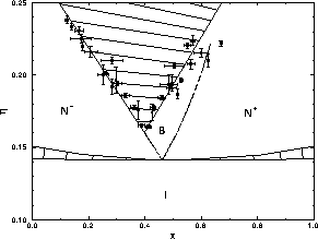
| Figure: | Computed phase diagram for a mixture of
prolate and oblate ellipsoids with an aspect ratio  =15. In
this figure, the phase diagram is shown in
the =15. In
this figure, the phase diagram is shown in
the  plane. Meaning of symbols as in figure
7.2. The location of the I-N
transition is obtained by matching the theoretical values of ref. [121] to
the simulation result for x=0.4. plane. Meaning of symbols as in figure
7.2. The location of the I-N
transition is obtained by matching the theoretical values of ref. [121] to
the simulation result for x=0.4. |
| Figure: | Typical snapshot of a NPT Monte Carlo simulation configuration in the biaxial phase. |
We found a clear phase separation for pressures higher than  =1.6, where
  is the proper volume of the particles. In figure 7.4 we show a snapshot of a demixed
configuration at high pressure. In figure 7.2 the
tentative phase diagram is displayed. The coexisting compositions are
plotted as a function of pressure for both the expansion and
compression. In figure 7.3 we plotted the phase
diagram as a function of the volume fraction
is the proper volume of the particles. In figure 7.4 we show a snapshot of a demixed
configuration at high pressure. In figure 7.2 the
tentative phase diagram is displayed. The coexisting compositions are
plotted as a function of pressure for both the expansion and
compression. In figure 7.3 we plotted the phase
diagram as a function of the volume fraction  . In both diagrams
the V-shaped two phase coexistence region is clearly visible and
resembles the theoretical
. In both diagrams
the V-shaped two phase coexistence region is clearly visible and
resembles the theoretical  =5 case, where there is no stable
biaxial phase. However, when we examined the nematic order parameters
in the coexisting phases, it appeared that the rod-rich mixture is not
a nematic
=5 case, where there is no stable
biaxial phase. However, when we examined the nematic order parameters
in the coexisting phases, it appeared that the rod-rich mixture is not
a nematic  phase but shows biaxial ordering. That is, both the
plate and rod nematic order parameter are large (
phase but shows biaxial ordering. That is, both the
plate and rod nematic order parameter are large ( 0.6) but
their corresponding directors are mutually perpendicular. A characteristic
simulation snapshot of a biaxial phase is shown in figure 7.5. The
compositions and volume fractions of the coexisting nematic
0.6) but
their corresponding directors are mutually perpendicular. A characteristic
simulation snapshot of a biaxial phase is shown in figure 7.5. The
compositions and volume fractions of the coexisting nematic  and
biaxial B phases have been collected
in table 7.1.
and
biaxial B phases have been collected
in table 7.1.
We also performed NPT simulations of rod-plate mixture at other
compositions between x=0.5 and x=0.8, to estimate the location of
the -continuous- phase transition from the biaxial to the nematic  phase. These estimates are indicated in figure 7.2
and 7.3 by a dotted line. Since, near the continuous
B-N
phase. These estimates are indicated in figure 7.2
and 7.3 by a dotted line. Since, near the continuous
B-N transition, fluctuations decay very slowly, the statistics of
the simulation results are
not very good and an accurate
location of the transition was not possible. In the phase diagram
we have also included a rough indication of the location of the isotropic to
nematic phase transition. As we only have an estimate for the I-N
transition for x=0.40 from the GEMC simulation results, we took the
coexistence region from the theoretical phase diagram of
ref. [121] and matched it
to the simulation result. Note, however, that this theoretical
coexistence curve is, by construction, symmetric whereas the true I-N
coexistence curve is likely to have a positive slope: due to the
presence of the higher virial coefficients, the I-N
transition for thin needles occurs at a higher pressure than
the corresponding transition for thin disks.
transition, fluctuations decay very slowly, the statistics of
the simulation results are
not very good and an accurate
location of the transition was not possible. In the phase diagram
we have also included a rough indication of the location of the isotropic to
nematic phase transition. As we only have an estimate for the I-N
transition for x=0.40 from the GEMC simulation results, we took the
coexistence region from the theoretical phase diagram of
ref. [121] and matched it
to the simulation result. Note, however, that this theoretical
coexistence curve is, by construction, symmetric whereas the true I-N
coexistence curve is likely to have a positive slope: due to the
presence of the higher virial coefficients, the I-N
transition for thin needles occurs at a higher pressure than
the corresponding transition for thin disks.
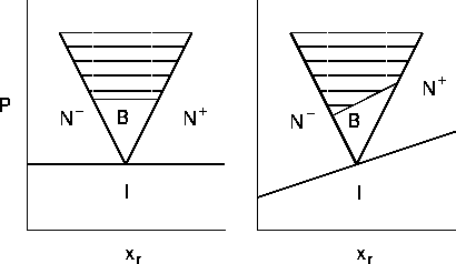
| Figure: | Rough sketch of the effect of rod-plate asymmetry on the theoretical phase diagram of ref. [121]. The figure on the left shows the phase diagram obtained in ref. [121] under the assumption that all virial coefficients higher than the second can be neglected. The figure on the right indicates the kind of asymmetry that could be induced in the phase diagram by the higher virial coefficients. Note that the figure on the right is qualitatively similar to figure 7.2. |
At first sight the phase diagrams obtained by simulation look rather different from the two theoretical scenarios shown in figure 7.1. The main difference is that the theoretical phase diagram is symmetric. However, this symmetry is an artifact and is due to the fact that, in the theory of ref. [121], higher virial coefficients were neglected. To be more precise, the particles considered by van Roij and Mulder have equal volumes and equal second virial coefficients. But the higher virial coefficients can differ significantly. For instance, the third virial coefficient of plates is larger than that of rods with the same second virial coefficient. One consequence is that the I-N transition for the pure rods is located at a higher density and pressure than that of plates. It is likely that the shape of the biaxial coexistence region will also be affected in the same way. One immediate consequence of any asymmetry in the theoretical phase-diagram would be that the average orientation of the biaxial-coexistence boundary would no longer be horizontal. In figure 7.6 we give an rough indication what lifting the symmetry requirement could do to the phase-diagram of ref. [121]. This figure illustrates that the simulated phase diagram is qualitatively similar to that predicted theoretically, once the spurious symmetry in the theoretical phase diagram is lifted.
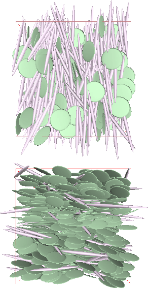
 phase, where
the plate director is free to move in the xy-plane. At the bottom
part the
phase, where
the plate director is free to move in the xy-plane. At the bottom
part the  phase is shown, in which there is no preferred
direction for the rods.
phase is shown, in which there is no preferred
direction for the rods.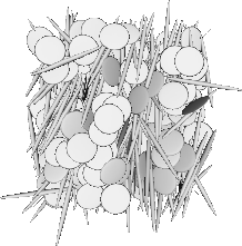
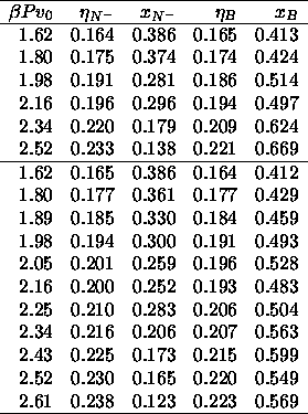
 =15.
The first sequence corresponds to expansion results, the
second to the compression. The pressure is expressed in units
=15.
The first sequence corresponds to expansion results, the
second to the compression. The pressure is expressed in units
 , where
  is the proper volume of the particles.