To gain a better intuitive understanding of the solid-solid transition in the square well model, it is instructive to compare the simulation results with a simple theoretical approach, vis. the uncorrelated cell model. The cell model is based on the idea that an atom in a solid is essentially confined to the ``cell'' formed by its nearest neighbors [64]. In the uncorrelated, single occupancy version of the cell model [65,66] the configurational part of the partition function of a N-particle system is approximated by
where  is the potential energy of the system, and
 is the potential energy of an atom and its nearest
neighbors. Here it is assumed that a cell can contain at most one
particle and that all correlations between cells can be ignored.
If one further assumes that every particle moves independently in a
regular fixed polyhedron formed by its neighbors fixed at their
lattice positions, the second integral of eqn.
3.11 can be
easily evaluated.
is the potential energy of an atom and its nearest
neighbors. Here it is assumed that a cell can contain at most one
particle and that all correlations between cells can be ignored.
If one further assumes that every particle moves independently in a
regular fixed polyhedron formed by its neighbors fixed at their
lattice positions, the second integral of eqn.
3.11 can be
easily evaluated.
We use the square-well model to describe the short ranged attractive
interaction.
Because the square well potential is a step function, the cell volume
can be divided into different regions characterized by the number of
neighbors within the range of its attractive well. The partition
function can now be expressed in terms of cell volume fractions
 in which the particle interacts with k particles simultaneously
where  is the parameter defined in eqn.
3.6, m
is the maximum number of neighbors and
is the parameter defined in eqn.
3.6, m
is the maximum number of neighbors and  the volume of the cell.
This volume depends on the dimensionality and the crystal structure.
For a three dimensional fcc structure the cell is a
dodecahedron with a volume
the volume of the cell.
This volume depends on the dimensionality and the crystal structure.
For a three dimensional fcc structure the cell is a
dodecahedron with a volume  , where a, the
radius of the cell, is defined as before
, where a, the
radius of the cell, is defined as before  .
In a two-dimensional triangular lattice,
.
In a two-dimensional triangular lattice, .
.
The Helmholtz free energy of the solid is given by the logarithm of
the partition function
The first term can be interpreted as the entropy of an ideal lattice gas, while the second term is the contribution due to the attractive interactions.
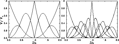
Figure 3.6 shows for the triangular and fcc
crystal structures the cell volume fraction  as a function of x.
For sufficiently short-ranged potentials,
the solid can be expanded to a density where a is much larger than
the width of the attractive
well
as a function of x.
For sufficiently short-ranged potentials,
the solid can be expanded to a density where a is much larger than
the width of the attractive
well  . In that case, a given particle can only have a few
neighbors within
the range of its attractive well. When the density is increased the
particle interacts with more neighbors. At
. In that case, a given particle can only have a few
neighbors within
the range of its attractive well. When the density is increased the
particle interacts with more neighbors. At  =1 the
particle has exactly half the number of neighbors within the
potential range. Once the density is so high that
=1 the
particle has exactly half the number of neighbors within the
potential range. Once the density is so high that  2,
then every particle interacts with all its nearest neighbors simultaneously.
This behavior leads to a fairly abrupt lowering of the potential
energy of the system.
2,
then every particle interacts with all its nearest neighbors simultaneously.
This behavior leads to a fairly abrupt lowering of the potential
energy of the system.
At low temperatures, this decrease of the energy on compression will
outweigh the loss of entropy that
is caused by the decrease of the free volume  .
The Helmholtz free energy F will then exhibit an inflection point,
and a first-order transition to a ``collapsed'' solid will result.
.
The Helmholtz free energy F will then exhibit an inflection point,
and a first-order transition to a ``collapsed'' solid will result.
By application of a double tangent construction we can compute the
coexisting densities as a function of temperature.
Figure 3.7 shows the coexistence curves in the
temperature density plane for different values of the attractive well
depth  . Indeed the cell model predicts a phase separation at
high density and small well width
. Indeed the cell model predicts a phase separation at
high density and small well width  .
The coexistence gap becomes larger when the temperature is lowered.
A spurious feature of this simple cell model is that it does not
predict a finite critical temperature. This stems from the fact that
in the cell model there is always a discontinuity in the pressure and
chemical potential that leads to a phase transition at all
temperatures. The discontinuity originates from the sharp change in
the volume fraction
.
The coexistence gap becomes larger when the temperature is lowered.
A spurious feature of this simple cell model is that it does not
predict a finite critical temperature. This stems from the fact that
in the cell model there is always a discontinuity in the pressure and
chemical potential that leads to a phase transition at all
temperatures. The discontinuity originates from the sharp change in
the volume fraction  at
at  (see figure
3.6) in the uncorrelated cell model approximation. As
the discontinuity of the pressure always takes place at a density
where
(see figure
3.6) in the uncorrelated cell model approximation. As
the discontinuity of the pressure always takes place at a density
where  , a very simple expression for the critical density
follows
, a very simple expression for the critical density
follows
where  denotes the density of the solid at regular close packing.
As can be seen in figure 3.8, the dependence of the
critical density on  obtained from the simulations is
described remarkably well by eqn.
3.14, despite the
fact that the finite critical temperature is not predicted by the
cell model calculations.
When all correlations are taken into account the discontinuities in
the free energy derivatives should disappear and a finite critical
temperature will result. Of course, more sophisticated cell model and
cell cluster theories that deal with the correlations
exists [57,67], but are not necessary for our purpose.
In a recent paper, Daanoun et al. [68] used a van der
Waals-like approximation to compute the phase diagram of a square-well
system. Although this approach also ignores all correlation effects,
these theoretical calculations reproduce the essential features of our
simulation data. Even better agreement has been found in recent
density-functional theory calculations by Likos et al. [69].
obtained from the simulations is
described remarkably well by eqn.
3.14, despite the
fact that the finite critical temperature is not predicted by the
cell model calculations.
When all correlations are taken into account the discontinuities in
the free energy derivatives should disappear and a finite critical
temperature will result. Of course, more sophisticated cell model and
cell cluster theories that deal with the correlations
exists [57,67], but are not necessary for our purpose.
In a recent paper, Daanoun et al. [68] used a van der
Waals-like approximation to compute the phase diagram of a square-well
system. Although this approach also ignores all correlation effects,
these theoretical calculations reproduce the essential features of our
simulation data. Even better agreement has been found in recent
density-functional theory calculations by Likos et al. [69].
 .
Top figure: two dimensional hexagonal lattice. The curves represent
from left to right, k=0,1...6.
Bottom figure: three dimensional fcc structure. From left to right
curves for k=0,1...12.
.
Top figure: two dimensional hexagonal lattice. The curves represent
from left to right, k=0,1...6.
Bottom figure: three dimensional fcc structure. From left to right
curves for k=0,1...12.


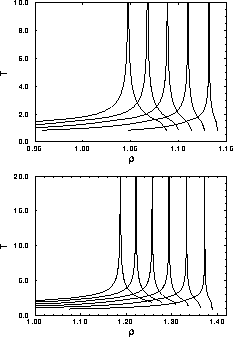
 plane
for the square well potential in the uncorrelated cell model
approximation. Top figure: Coexistence curves for a two dimensional
hexagonal lattice. From right to left
plane
for the square well potential in the uncorrelated cell model
approximation. Top figure: Coexistence curves for a two dimensional
hexagonal lattice. From right to left  =0.01, 0.02,
0.03, 0.04 and 0.05. Bottom figure: Coexistence curves for a three
dimensional fcc lattice. From right to left
=0.01, 0.02,
0.03, 0.04 and 0.05. Bottom figure: Coexistence curves for a three
dimensional fcc lattice. From right to left  =0.01,
0.02, 0.03, 0.04, 0.05 and 0.06. In both figures no critical
temperature is obtained due to discontinuities in the derivatives of
the cell model free energy.
=0.01,
0.02, 0.03, 0.04, 0.05 and 0.06. In both figures no critical
temperature is obtained due to discontinuities in the derivatives of
the cell model free energy.
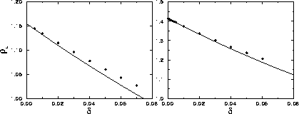
 . The circles denote the
simulation results, while the solid curve denotes the prediction of
the uncorrelated cell model.
The upper figure refers to two dimensions while the lower figure
shows the three dimensional case.
. The circles denote the
simulation results, while the solid curve denotes the prediction of
the uncorrelated cell model.
The upper figure refers to two dimensions while the lower figure
shows the three dimensional case.